SPONGE Enhanced Sampling Example
SPONGE 1.4 tutorial.This page was translated by GPT-5.5 AI.
SPONGE Enhanced Sampling Example
Last updated:
2024/01/01
Program Installation
See Installation on Linux and Installation on Windows.
What Is Enhanced Sampling?
Usually, our molecular dynamics (MD) simulations are performed under a given force field with a potential energy function
If the required result cannot be obtained under this potential energy function, an enhanced sampling algorithm can be used. In this case, a manually defined bias potential is added to the potential energy function:
A simulation with an added bias potential is, of course, different from the real unbiased simulation, but the result can be transformed through calculation. The theoretical basis is the distribution function of thermodynamic quantities in each ensemble. For example, in the canonical ensemble,
Therefore, each occurrence probability in the simulation result only needs to be reweighted, that is, multiplied by ${\rm exp}(\beta U_{bias}(x))$:
Why Use Enhanced Sampling?
Here, we build a hydrogen peroxide model system. After decompression, the file directory is as follows:
│  H2O2_angle.txt
│  H2O2_bond.txt
│  H2O2_charge.txt
│  H2O2_coordinate.txt
│  H2O2_dihedral.txt
│  H2O2_exclude.txt
│  H2O2_LJ.txt
│  H2O2_mass.txt
│  H2O2_nb14.txt
│  H2O2_residue.txt
│
├─bad_normal_md
│      analysis.py
│      cv.txt
│      H2O2_dihedral.txt
│      mdin.txt
│
├─metadynamics
│      analysis.py
│      cv.txt
│      H2O2_dihedral.txt
│      mdin.txt
│
├─normal_md
│      analysis.py
│      cv.txt
│      mdin.txt
│
├─sits
│      analysis.py
│      cv.txt
│      H2O2_dihedral.txt
│      iteration.in
│      observation.in
│      production.in
│
└─umbrella_sampling
        analysis.py
        cv.txt
        H2O2_dihedral.txt
        min.in
        run.in
        run.py
In this model system, I removed the LJ and electrostatic interactions of hydrogen peroxide and kept only the potential energy terms for internal coordinates such as bond lengths, bond angles, and dihedral angles. This makes the example simpler and makes it easier to understand the principle and program usage.
Open the H2O2_dihedral.txt file:
2
2 0 1 3 2 0.3 0.4
2 0 1 3 3 0.1 -0.6
According to the file formats and module functions in the SPONGE documentation, we know that this corresponds to the potential energy function
First, enter the normal_md folder in the archive and run SPONGE directly in this folder.
SPONGE -mdin mdin.txt
In our mdin, the CV input file is set to cv.txt, whose content is
print
{
    CV = torsion
}
torsion
{
   CV_type = dihedral
   atom = 2 0 1 3
}
Here we define a CV named torsion. Its type is dihedral, and the parameter atoms are 2, 0, 1, and 3.
After the simulation finishes, the output file mdout.txt is generated. We use the following Python script (analysis.py in this directory) for analysis:
from Xponge.analysis import MdoutReader
import numpy as np
import matplotlib.pyplot as plt
from scipy.stats import gaussian_kde
t = MdoutReader("mdout.txt")
t = t.torsion
kT = 8.314 * 300 / 4184
t = np.concatenate((t, t + np.pi * 2, t - np.pi * 2))
kernel = gaussian_kde(t, bw_method=0.03)
positions = np.linspace(-np.pi, np.pi, 300)
result = kernel(positions)
result = -kT * np.log(result)
result -= min(result)
theory = 0.3 * np.cos(2 * positions - 0.4) + 0.1 * np.cos(3 * positions + 0.6)
theory -= min(theory)
plt.plot(positions, result, label="simulated results")
plt.plot(positions, theory, label="potential")
plt.legend()
plt.show()
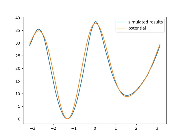
The potential energy surface obtained from the simulation is roughly consistent with the specified dihedral energy. Although the result is still not fully satisfactory, it should become better if we increase the simulation time by a limited amount.
Now enter the bad_normal_md folder. In this folder, our mdin specifies a file that replaces the default dihedral file. Its content is
2
2 0 1 3 2 15 0.4
2 0 1 3 3 5 -0.6
The potential energy function has been multiplied directly by 50. At this point, room temperature is not enough for this artificial hydrogen peroxide system to cross the dihedral barrier.
Next, run an MD simulation for the same length of time.
SPONGE -mdin mdin.txt
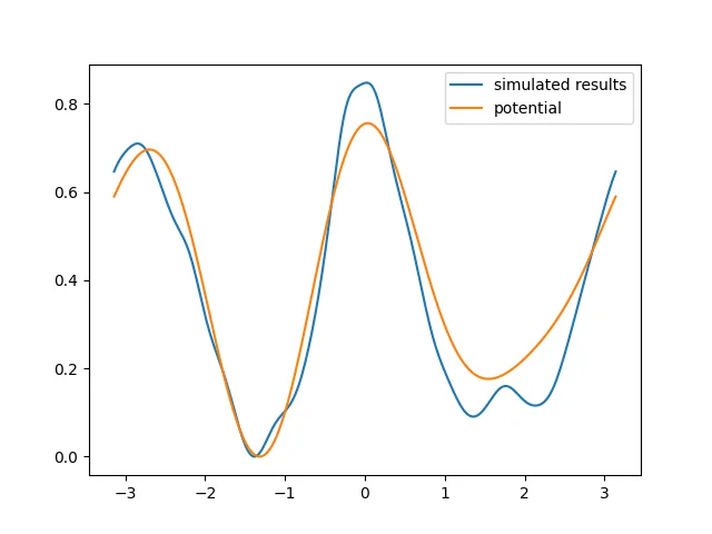
Analyze it with the same script as above. The result is as follows:
It can be seen that the simulation result is now very poor, so an enhanced sampling algorithm is needed.
Umbrella Sampling
Enter the umbrella_sampling folder. First, look at the cv.txt file:
print
{
    CV = torsion
}
torsion
{
   CV_type = dihedral
   atom = 2 0 1 3
}
restrain
{
    CV = torsion
    weight = 200
    reference = res_cv_ref
    period = 6.283185308
}
Compared with the cv.txt used in normal MD, this file adds a restrain section, which applies a harmonic restraint. The reference value is set to res_cv_ref, which is specified by external input.
Write the Python script run.py to run the jobs in batches:
import os
import shutil
import numpy as np
for i, ref in enumerate(np.linspace(-np.pi,np.pi,50)):
    assert os.system(f"SPONGE -mdin min.in -res_cv_ref {ref}") == 0
    assert os.system(f"SPONGE -mdin run.in -res_cv_ref {ref} -coordinate_in_file restart_coordinate.txt") == 0
    shutil.copy("mdout.txt", f"{i}.mdout")
python run.py
Finally, 50 mdout files are obtained.
For umbrella sampling, because the trajectories involve many bias potentials, the WHAM algorithm is required for reweighting. We use the following script for analysis:
import numpy as np
import matplotlib.pyplot as plt
from Xponge.analysis import wham
"""use help(wham.WHAM) to see the help"""
w = wham.WHAM(np.linspace(-np.pi, np.pi, 51), 300, 200, np.linspace(-np.pi, np.pi, 50), 2 * np.pi)
w.get_data_from_mdout("*.mdout", "torsion")
x, y, f = w.main()
plt.plot(x, y, label="umbrella sampling")
y2 = 15 * np.cos(2 * x - 0.4) + 5 * np.cos(3 * x + 0.6)
y2 -= min(y2)
plt.plot(x, y2, label="potential")
plt.legend()
plt.show()
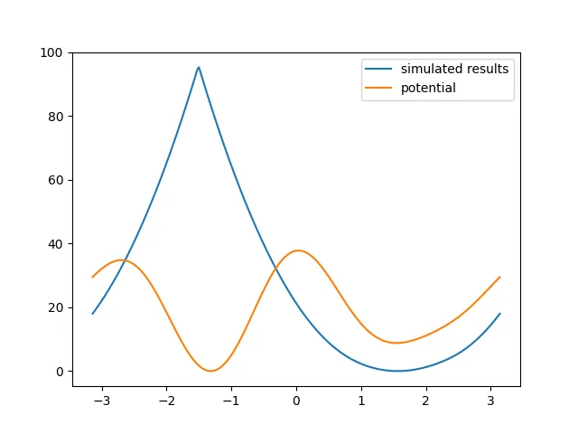
The final result is
The effect is good.
Metadynamics
Enter the metadynamics folder. First, look at the cv.txt file:
print
{
    CV = torsion
}
torsion
{
   CV_type = dihedral
   atom = 2 0 1 3
}
meta1d
{
    CV = torsion
    dCV = 0.001
    CV_minimal = -3.142
    CV_maximum = 3.142
    CV_period = 6.284
    welltemp_factor = 50
    height = 1
    sigma = 0.5
}
Compared with the cv.txt used in normal MD, this file adds a meta1d section. For the specific meanings of the settings, see the SPONGE documentation.
Next, run an MD simulation for the same length of time.
SPONGE -mdin mdin.txt
Use the following script to analyze the result:
from Xponge.analysis import MdoutReader
import numpy as np
import matplotlib.pyplot as plt
from scipy.stats import gaussian_kde
t = MdoutReader("mdout.txt")
bias = t.meta1d
t = t.torsion
kT = 8.314 * 300 / 4184
w = np.exp(bias/kT)
t = np.concatenate((t, t + np.pi * 2, t - np.pi * 2))
w = np.concatenate((w, w, w))
kernel = gaussian_kde(t, weights=w, bw_method=0.01)
positions = np.linspace(-np.pi, np.pi, 300)
result = kernel(positions)
result = -kT * np.log(result)
result -= min(result)
theory = 15 * np.cos(2 * positions - 0.4) + 5 * np.cos(3 * positions + 0.6)
theory -= min(theory)
plt.plot(positions, result, label="simulated results")
plt.plot(positions, theory, label="potential")
toread = np.loadtxt("meta1d_potential.txt", skiprows=3)
toread[:, 1] = -toread[:, 1]
toread[:, 1] -= np.min(toread[:, 1])
plt.plot(toread[:, 0], toread[:, 1], label="meta1d potential")
plt.legend()
plt.show()
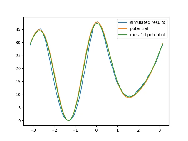
Two ways of obtaining the result are used here. One is reweighting, and the other is directly using the negative of the potential energy function added by metadynamics. In this example, both methods give the same effect.
When obtaining the free energy surface from the negative of the potential energy function added by metadynamics, an additional factor is actually required because well-tempered metadynamics is used. This factor is
Here this factor is $\frac {50} {0.596148 + 50} \approx 1$.
Selective Integrated Tempering Sampling
Note that this example is essentially a CV sampling example and is not very suitable for SITS, but the principle is the same.
Observation
First, we need to observe the system.
SPONGE -mdin observation.in
In this input file, the additional commands are
SITS
{
    mode = observation
    atom_numbers = 4
}
sits_dihedral_in_file = H2O2_dihedral.txt
Here, SITS_mode = observation means observation, SITS_atom_numbers = 4 means that ITS is applied to the nonbonded interactions of the first 4 atoms, and sits_dihedral_in_file specifies the dihedral angle on which we want to perform ITS.
During the run, we mainly observe the SITS_AA_kAB part, which is the energy that we ultimately want to enhance. We set pe_b according to the minimum value observed for this quantity minus an estimated retained value.
In this example, SITS_AA_kAB is around 9. We estimate that the later value may decrease by 20, so pe_b is set to -(9 - 20) = 11.
The choice of
pe_bis system-dependent. You need to tunepe_breasonably; otherwise, the system is very likely to crash!
Next, perform the iteration step.
SPONGE -mdin iteration.in
In this input file, the additional commands are
SITS
{
    mode = iteration
    atom_numbers = 4
    T_high = 8000
    k_numbers = 8000
    T_low = 200
    pe_b = 11
}
sits_dihedral_in_file = H2O2_dihedral.txt
This section adds the highest temperature for integration, the lowest temperature for integration, the number of discrete grid points for integration, and the pe_b mentioned above. These parameters can all be adjusted, but poor parameters may cause abrupt changes in the potential energy function and then crash the simulation.
After this simulation step, the most important result is the SITS_nk_rest.txt file, which contains free energy information at different temperatures. We use this file for the production simulation.
SPONGE -mdin production.in
In this input file, the additional commands are
SITS
{
    mode = production
    atom_numbers = 4
    T_high = 8000
    k_numbers = 8000
    T_low = 200
    pe_b = 11
    nk_in_file = SITS_nk_rest.txt
}
sits_dihedral_in_file = H2O2_dihedral.txt
The new part here is that SITS_nk_rest.txt, obtained in the iteration step, is used as input and passed to the nk_in_file command.
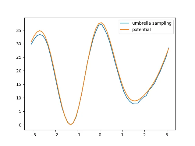
After the simulation finishes, use the following script for analysis:
from Xponge.analysis import MdoutReader
import numpy as np
import matplotlib.pyplot as plt
from scipy.stats import gaussian_kde
t = MdoutReader("mdout.txt")
bias = t.SITS_bias
t = t.torsion
kT = 8.314 * 300 / 4184
w = np.exp(bias/kT)
t = np.concatenate((t, t + np.pi * 2, t - np.pi * 2))
w = np.concatenate((w, w, w))
kernel = gaussian_kde(t, weights=w, bw_method=0.01)
positions = np.linspace(-np.pi, np.pi, 300)
result = kernel(positions)
result = -kT * np.log(result)
result -= min(result)
theory = 15 * np.cos(2 * positions - 0.4) + 5 * np.cos(3 * positions + 0.6)
theory -= min(theory)
plt.plot(positions, result, label="simulated results")
plt.plot(positions, theory, label="potential")
plt.legend()
plt.show()
The result is as follows: