SPONGE增强抽样案例

更新时间：
2024/01/01

程序安装

见Linux下的安装和Windows下的安装

什么是增强抽样？

通常，我们的分子动力学（MD）模拟在某一力场下进行，有势能函数

$$U(x)U(x)$$

在该势能函数下，如果我们得不到需要的结果，此时可以使用增强抽样算法，在势能函数上添加上我们人为设定的偏置势（bias）

$$U^{\mathrm{\prime }}(x)=U(x)+U_{bias}(x)U\text{'}(x)\; =\; U(x)\; +\; U\_\{bias\}\; (x)$$

添加偏置势的模拟当然和真实模拟不同，但是可以根据计算进行转化，其理论基础是各系综下热力学量的分布函数计算，例如正则系综下有

$$p(x)=\frac{1}{Q}\mathrm{e}\mathrm{x}\mathrm{p}(-\beta U(x))p(x)\; =\; \backslash frac\; \{1\}\{Q\}\; \{\backslash rm\; exp\}(-\backslash beta\; U(x))$$

这样我们模拟得到的结果每个出现的概率均做一个重加权即可，也即乘上$\mathrm{e}\mathrm{x}\mathrm{p}(\beta U_{bias}(x))\{\backslash rm\; exp\}(\backslash beta\; U\_\{bias\}(x))$

$$p^{\mathrm{\prime }}(x)=\frac{1}{Q}\mathrm{e}\mathrm{x}\mathrm{p}(-\beta U^{\mathrm{\prime }}(x))=\frac{1}{Q}\mathrm{e}\mathrm{x}\mathrm{p}(-\beta (U(x)+U_{bias}(x)))=p(x)\mathrm{e}\mathrm{x}\mathrm{p}(-\beta U_{bias}(x))p\text{'}(x)\; =\; \backslash frac\; \{1\}\{Q\}\; \{\backslash rm\; exp\}(-\backslash beta\; U\text{'}(x))\; =\; \backslash frac\; \{1\}\{Q\}\; \{\backslash rm\; exp\}(-\backslash beta\; (U(x)\; +\; U\_\{bias\}(x)))\; =\; p(x)\; \{\backslash rm\; exp\}(-\backslash beta\; U\_\{bias\}(x))$$

为什么使用增强抽样

这里，我们构建一个过氧化氢的模型体系，解压后的文件目录下为

│  H2O2_angle.txt
│  H2O2_bond.txt
│  H2O2_charge.txt
│  H2O2_coordinate.txt
│  H2O2_dihedral.txt
│  H2O2_exclude.txt
│  H2O2_LJ.txt
│  H2O2_mass.txt
│  H2O2_nb14.txt
│  H2O2_residue.txt
│
├─bad_normal_md
│      analysis.py
│      cv.txt
│      H2O2_dihedral.txt
│      mdin.txt
│
├─metadynamics
│      analysis.py
│      cv.txt
│      H2O2_dihedral.txt
│      mdin.txt
│
├─normal_md
│      analysis.py
│      cv.txt
│      mdin.txt
│
├─sits
│      analysis.py
│      cv.txt
│      H2O2_dihedral.txt
│      iteration.in
│      observation.in
│      production.in
│
└─umbrella_sampling
        analysis.py
        cv.txt
        H2O2_dihedral.txt
        min.in
        run.in
        run.py

这个模型体系中，我取消掉了过氧化氢的LJ和静电，只保留了键长、键角、二面角等内坐标的势能，让例子更简单以更方便了解原理和程序使用。

我们查看H2O2_dihedral.txt文件，有

2
2 0 1 3 2 0.3 0.4
2 0 1 3 3 0.1 -0.6

根据SPONGE文档中的文件格式和模块功能，我们可以知道这相当于势能函数

$$U(\varphi )=0.3(1+cos(2\varphi -0.4))+0.1(1+cos(3\varphi +0.6))U(\backslash phi)\; =\; 0.3\; (1\; +\; cos(2\backslash phi\; -\; 0.4))\; +\; 0.1\; (1\; +\; cos(3\backslash phi\; +\; 0.6))$$

首先我们进入到压缩文件的normal_md文件夹中，在该文件夹中直接运行SPONGE。

SPONGE -mdin mdin.txt

在我们的mdin中，我们设置了我们的cv输入文件是cv.txt，其内容是

print
{
    CV = torsion
}
torsion
{
   CV_type = dihedral
   atom = 2 0 1 3
}

我们在其中定义了一个名叫torsion，类型为dihedral，参数原子是2、0、1、3的CV

模拟结束过后，得到结果文件mdout.txt，我们使用以下python脚本（该目录下的analysis.py）进行分析

from Xponge.analysis import MdoutReader
import numpy as np
import matplotlib.pyplot as plt
from scipy.stats import gaussian_kde
t = MdoutReader("mdout.txt")
t = t.torsion
kT = 8.314 * 300 / 4184
t = np.concatenate((t, t + np.pi * 2, t - np.pi * 2))
kernel = gaussian_kde(t, bw_method=0.03)
positions = np.linspace(-np.pi, np.pi, 300)
result = kernel(positions)
result = -kT * np.log(result)
result -= min(result)
theory = 0.3 * np.cos(2 * positions - 0.4) + 0.1 * np.cos(3 * positions + 0.6)
theory -= min(theory)
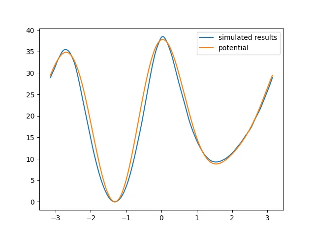
plt.plot(positions, result, label="simulated results")
plt.plot(positions, theory, label="potential")
plt.legend()
plt.show()

可见模拟得到的势能面与设定的二面角能量大致一致。虽然结果仍然不尽如人意，但是相信如果我们增加有限的模拟时长就能获得更好的采样结果。

那么我们现在进入bad_normal_md文件夹中，在这个文件夹中，我们的mdin中指定了替代默认dihedral的文件，在该文件中

2
2 0 1 3 2 15 0.4
2 0 1 3 3 5 -0.6

$$U(\varphi )=15(1+cos(2\varphi -0.4))+5(1+cos(3\varphi +0.6))U(\backslash phi)\; =\; 15\; (1\; +\; cos(2\backslash phi\; -\; 0.4))\; +\; 5\; (1\; +\; cos(3\backslash phi\; +\; 0.6))$$

我们的势能函数直接乘了50，此时室温并不足以使得这个虚假的过氧化氢翻过二面角势垒

我们接下来也跑相同时间的MD模拟

SPONGE -mdin mdin.txt

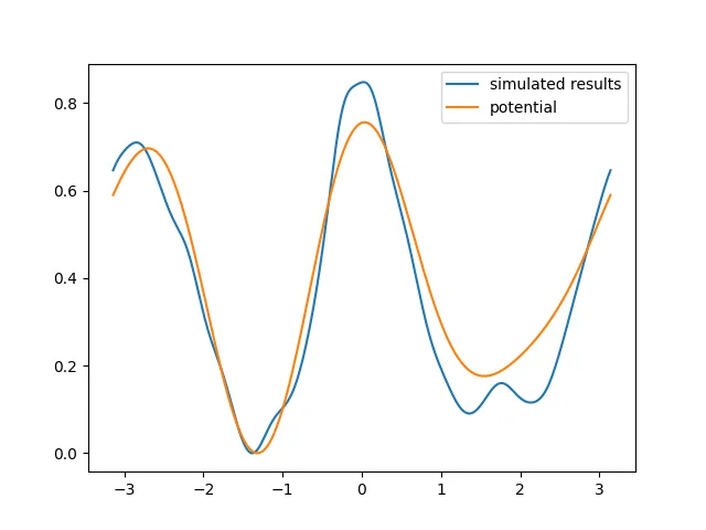
用上面相同脚本分析，得到结果如下：

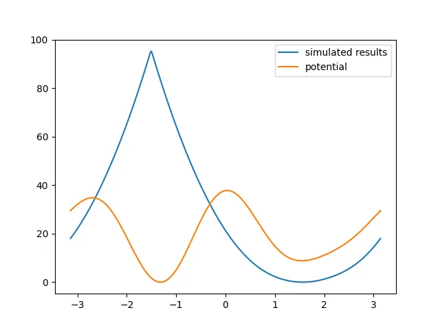
可见，此时模拟得到的结果已经非常不好，需要使用增强抽样算法。

伞形抽样

进入umbrella_sampling文件夹中，我们首先看看我们的cv.txt文件

print
{
    CV = torsion
}
torsion
{
   CV_type = dihedral
   atom = 2 0 1 3
}
restrain
{
    CV = torsion
    weight = 200
    reference = res_cv_ref
    period = 6.283185308
}

这里，除了和普通md里一样的cv.txt以外，还加入了restrain部分，也就是简谐势限制。其中的参考值设为了res_cv_ref，由外部输入指定

编写python脚本run.py批量运行

import os
import shutil
import numpy as np
for i, ref in enumerate(np.linspace(-np.pi,np.pi,50)):
    assert os.system(f"SPONGE -mdin min.in -res_cv_ref {ref}") == 0
    assert os.system(f"SPONGE -mdin run.in -res_cv_ref {ref} -coordinate_in_file restart_coordinate.txt") == 0
    shutil.copy("mdout.txt", f"{i}.mdout")

python run.py

最后获得了50份mdout

对于umbrella sampling，因为轨迹涉及很多个bias，需要使用WHAM算法重加权。我们使用下列脚本分析

import numpy as np
import matplotlib.pyplot as plt
from Xponge.analysis import wham
"""use help(wham.WHAM) to see the help"""
w = wham.WHAM(np.linspace(-np.pi, np.pi, 51), 300, 200, np.linspace(-np.pi, np.pi, 50), 2 * np.pi)
w.get_data_from_mdout("*.mdout", "torsion")
x, y, f = w.main()
plt.plot(x, y, label="umbrella sampling")
y2 = 15 * np.cos(2 * x - 0.4) + 5 * np.cos(3 * x + 0.6)
y2 -= min(y2)
plt.plot(x, y2, label="potential")
plt.legend()
plt.show()

最终得到的结果为

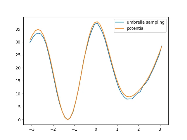
可见效果较好

埋拓动力学

进入umbrella_sampling文件夹中，我们首先看看我们的cv.txt文件

print
{
    CV = torsion
}
torsion
{
   CV_type = dihedral
   atom = 2 0 1 3
}
meta1d
{
    CV = torsion
    dCV = 0.001
    CV_minimal = -3.142
    CV_maximum = 3.142
    CV_period = 6.284
    welltemp_factor = 50
    height = 1
    sigma = 0.5
}

这里，除了和普通md里一样的cv.txt以外，还加入了meta1d部分。具体含义可查询SPONGE文档

我们接下来也跑相同时间的MD模拟

SPONGE -mdin mdin.txt

使用下列脚本进行分析结果

from Xponge.analysis import MdoutReader
import numpy as np
import matplotlib.pyplot as plt
from scipy.stats import gaussian_kde
t = MdoutReader("mdout.txt")
bias = t.meta1d
t = t.torsion
kT = 8.314 * 300 / 4184
w = np.exp(bias/kT)
t = np.concatenate((t, t + np.pi * 2, t - np.pi * 2))
w = np.concatenate((w, w, w))
kernel = gaussian_kde(t, weights=w, bw_method=0.01)
positions = np.linspace(-np.pi, np.pi, 300)
result = kernel(positions)
result = -kT * np.log(result)
result -= min(result)
theory = 15 * np.cos(2 * positions - 0.4) + 5 * np.cos(3 * positions + 0.6)
theory -= min(theory)
plt.plot(positions, result, label="simulated results")
plt.plot(positions, theory, label="potential")
toread = np.loadtxt("meta1d_potential.txt", skiprows=3)
toread[:, 1] = -toread[:, 1]
toread[:, 1] -= np.min(toread[:, 1])
plt.plot(toread[:, 0], toread[:, 1], label="meta1d potential")
plt.legend()
plt.show()

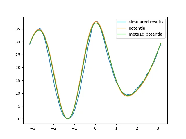
这里使用了两种得到结果的方式，一种是重加权，另外一种是直接使用metadynamics添加的势能函数的相反数，两种方式在此例中得到的效果相同。

使用metadynamics添加的势能函数的相反数得到自由能曲面时，因为使用了well-tempered metadynamics，所以实际上还要乘上一个因子，这个因子为

$$\frac{\mathrm{w}\mathrm{e}\mathrm{l}\mathrm{l}\mathrm{t}\mathrm{e}\mathrm{m}\mathrm{p}\mathrm{\_}\mathrm{f}\mathrm{a}\mathrm{c}\mathrm{t}\mathrm{o}\mathrm{r}}{k_{B}T+\mathrm{w}\mathrm{e}\mathrm{l}\mathrm{l}\mathrm{t}\mathrm{e}\mathrm{m}\mathrm{p}\mathrm{\_}\mathrm{f}\mathrm{a}\mathrm{c}\mathrm{t}\mathrm{o}\mathrm{r}}\backslash frac\; \{\backslash rm\; welltemp\backslash \_factor\}\; \{k\_B\; T\; +\; \{\backslash rm\; welltemp\backslash \_factor\}\}$$

这里该因子$=\frac{50}{0.596148+50}\approx 1=\backslash frac\; \{50\}\; \{0.596148\; +\; 50\}\; \backslash approx1$

选择性温度积分增强抽样

注意，这里的例子本质是一个针对CV的抽样例子，并不太适合SITS，但原理是相同的

观察

首先，我们需要观察我们的体系。

SPONGE -mdin observation.in

在这个in文件里，我们加入了的额外命令是

SITS
{
    mode = observation
    atom_numbers = 4
}
sits_dihedral_in_file = H2O2_dihedral.txt

其中，SITS_mode = observation 表示观察，SITS_atom_numbers = 4表示我们对前4个原子的非键作用进行ITS，而sits_dihedral_in_file则指明我们希望进行ITS的二面角
运行时，我们主要观察其中的SITS_AA_kAB这一部分，这一部分是我们最终希望增强的能量。我们根据这个值的最小出现的值，减去一个预估的保留值，设置pe_b。
如此处，SITS_AA_kAB为9左右，我们预估后面会降低的值为20，设置的pe_b因此为-(9-20) = 11。

这里的pe_b选择是基于体系的。你需要合理调节pe_b的值，否则系统很有可能出现崩溃!

接下来，我们就进行迭代处理

SPONGE -mdin iteration.in

在这个in文件里，我们加入了的额外命令是

SITS
{
    mode = iteration
    atom_numbers = 4
    T_high = 8000
    k_numbers = 8000
    T_low = 200
    pe_b = 11
}
sits_dihedral_in_file = H2O2_dihedral.txt

这个部分新增包括积分的最高温度、积分的最低温度和积分的离散格点数，以及上面提到的pe_b。这些参数都是可以调节的，而较差的参数可能会引起势能函数突变，进而模拟崩溃。

该步模拟后，最重要的就是获得SITS_nk_rest.txt文件，该文件包含了不同温度的自由能信息，我们用该文件进行生产模拟

SPONGE -mdin production.in

在这个in文件里，我们加入了的额外命令是

SITS
{
    mode = production
    atom_numbers = 4
    T_high = 8000
    k_numbers = 8000
    T_low = 200
    pe_b = 11
    nk_in_file = SITS_nk_rest.txt
}
sits_dihedral_in_file = H2O2_dihedral.txt

这部分新增加的就是iteration部分获得的SITS_nk_rest.txt作为输入，给到nk_in_file命令。

模拟结束后使用下列脚本进行分析

from Xponge.analysis import MdoutReader
import numpy as np
import matplotlib.pyplot as plt
from scipy.stats import gaussian_kde
t = MdoutReader("mdout.txt")
bias = t.SITS_bias
t = t.torsion
kT = 8.314 * 300 / 4184
w = np.exp(bias/kT)
t = np.concatenate((t, t + np.pi * 2, t - np.pi * 2))
w = np.concatenate((w, w, w))
kernel = gaussian_kde(t, weights=w, bw_method=0.01)
positions = np.linspace(-np.pi, np.pi, 300)
result = kernel(positions)
result = -kT * np.log(result)
result -= min(result)
theory = 15 * np.cos(2 * positions - 0.4) + 5 * np.cos(3 * positions + 0.6)
theory -= min(theory)
plt.plot(positions, result, label="simulated results")
plt.plot(positions, theory, label="potential")
plt.legend()
plt.show()

得到结果如下：