This page was translated by GPT-5.5 AI.

Simulation of Sodium Chloride Crystals

Introduction

This tutorial mainly reproduces the core simulation part of a paper published in Acta Physica Sinica.

Shouxin Cui, Lingcang Cai, Haiquan Hu, Yongxin Guo, Shikai Xiang, Fuqian Jing. Molecular dynamics calculation of thermophysical parameters of sodium chloride crystals under high temperature and high pressure. Acta Physica Sinica, 2005, 54(6): 2826-2831. doi: 10.7498/aps.54.2826

Model Building

The force field used in the original paper is relatively complex. This tutorial only discusses basic MD and is not intended to fully reproduce the reported results, so the force field used here is the sodium ion and chloride ion force field bundled with the TIP3P water model in Xponge.

In Suk Joung and Thomas E. Cheatham, Determination of Alkali and Halide Monovalent Ion Parameters for Use in Explicitly Solvated Biomolecular Simulations, The Journal of Physical Chemistry B 2008 112 (30), 9020-9041, DOI: 10.1021/jp8001614

Following the original paper,

use Xponge for model building. Write the Python script build.py as follows:

# Import the Xponge module
import Xponge
# Import the force field
import Xponge.forcefield.amber.tip3p
# Define the structural unit: NA at (0,0,0) and CL at (4,0,0)
# The 4 Angstrom value is arbitrary here; it only needs to avoid an overly short distance.
# The MD simulation will equilibrate it to the correct position.
mol0 = NA + CL
mol0.residues[-1].CL.x = 4
# Define the cubic fill region from (0,0,0) to (64,64,64)
region = Xponge.BlockRegion(0, 0, 0, 64, 64, 64)
# Define the periodic box from (0,0,0) to (70,70,70)
box = Xponge.BlockRegion(0, 0, 0, 65, 65, 65)
# Define the lattice: an fcc crystal with an 8 Angstrom unit-lattice spacing
lattice = Xponge.Lattice("fcc", mol0, 8)
# Create the cells
mol = lattice.Create(box, region)
# Save the files
Save_PDB(mol, "NaCl.pdb")
Save_SPONGE_Input(mol, "NaCl")

Run the following commands in the command line:

python build.py
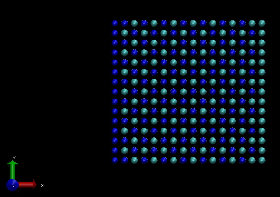
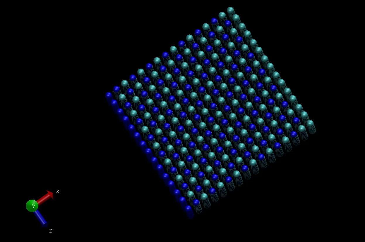
vmd NaCl.pdb

After adjusting several visualization settings, the following visualization results are obtained:

Molecular Dynamics Simulation

Minimization

Enter the following command in the command line to perform 5000 steps of gradient-descent minimization:

SPONGE -default_in_file_prefix NaCl -mode minimization -step_limit 5000 -rst min

The meaning of each part is as follows:

• SPONGE
  The CUDA SPONGE program
• -default_in_file_prefix NaCl
  The default prefix of the input files is NaCl, corresponding to Save_SPONGE_Input(mol, “NaCl”) in the model-building process
• -mode minimization
  Run minimization, using the variable-step-size gradient descent algorithm by default
• -step_limit 5000
  The total number of steps is 5000
• -rst min
  The prefix of the generated coordinate and velocity files is min. That is, the generated coordinate file is min_coordinate.txt, and the generated velocity file is min_velocity.txt (the velocity file has no obvious significance for minimization)

NPT Simulation at 300 K and 40 GPa

Enter the following command in the command line to perform a 50000-step NPT ensemble simulation:

SPONGE -default_in_file_prefix NaCl -coordinate_in_file min_coordinate.txt -mode NPT -dt 1e-3 -step_limit 55000 -thermostat middle_langevin -middle_langevin_gamma 10 -barostat berendsen_barostat -target_temperature 300 -target_pressure 400000 -mdout 40GPa.out -rst 40GPa -crd 40GPa.dat -box 40GPa.box

The meaning of each part is as follows:

• SPONGE
  The CUDA SPONGE program
• -default_in_file_prefix NaCl
  The default prefix of the input files is NaCl, corresponding to Save_SPONGE_Input(mol, “NaCl”) in the model-building process
• -coordinate_in_file min_coordinate.txt
  Use the coordinates from the minimization result as the initial coordinates for the simulation
• -mode NPT
  Run an NPT simulation
• -dt 1e-3
  The simulation time step is 1e-3 ps, namely 1 fs
• -step_limit 5000
  The total number of steps is 50000
• -thermostat middle_langevin
  Use the middle Langevin method for temperature control
• -middle_langevin_gamma 10
  The temperature-control frequency is 10 ps^-1. Note that the default value here is 1. Because the pressure in this simulation is very high, the default frequency may be too low to keep the temperature under control
• -barostat berendsen_barostat
  Use the Berendsen method for pressure control
• -target_temperature 300
  Control the temperature to 300 K
• -target_pressure 400000
  Control the pressure to 400000 bar (40 GPa)
• -mdout 40GPa.out
  Write the log file to 40GPa.out

NPT Simulation at 300 K and 0 GPa

Enter the following command in the command line to perform a 50000-step NPT ensemble simulation. Here, the result obtained at 40 GPa is used as the input condition.

SPONGE -default_in_file_prefix NaCl -coordinate_in_file 40GPa_coordinate.txt -velocity_in_file 40GPa_velocity.txt -mode NPT -dt 1e-3 -step_limit 55000 -thermostat middle_langevin -middle_langevin_gamma 10 -barostat berendsen_barostat -target_temperature 300 -target_pressure 1 -mdout 0GPa.out  -crd 0GPa.dat -box 0GPa.box

The meanings of the options are the same as above, except that the additional command -velocity_in_file 40GPa_velocity.txt is added to provide the initial velocities.

Analysis and Discussion

Trajectory Visualization

Use VMD for visualization. The 40 GPa trajectory is used as an example:

vmd -sponge_mass NaCl_mass.txt 40GPa.dat

Result Analysis

Write the analysis script analysis.py:

import numpy as np
import matplotlib.pyplot as plt
import Xponge
from Xponge.analysis import MdoutReader
mdout1 = MdoutReader("0GPa.out")
mdout2 = MdoutReader("40GPa.out")
plt.plot(mdout1.time, mdout1.density, label="0 GPa")
plt.plot(mdout1.time, mdout2.density, label="40 GPa")
plt.legend()
plt.show()
density1 = np.mean(mdout1.density)
density2 = np.mean(mdout2.density)
print(density1, density2, density1/density2)

The results are as follows:

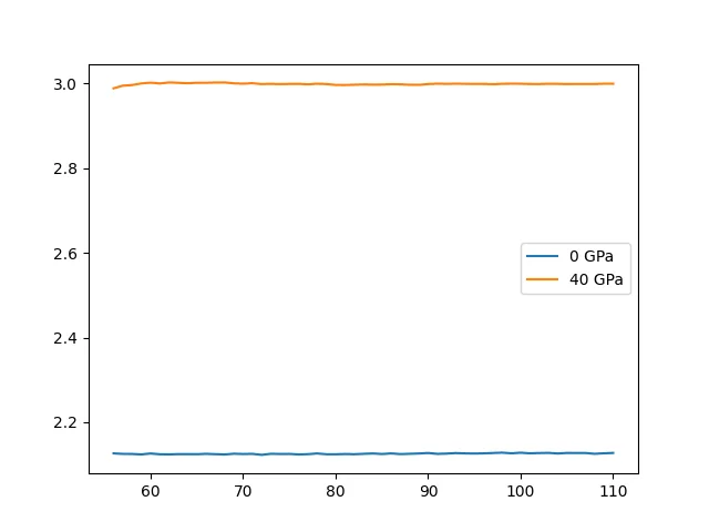
The average densities are $2.126\mathrm{g}\mathrm{/}\mathrm{c}{\mathrm{m}}^{-3}2.126\backslash ,\{\backslash rm\; g/cm^\{-3\}\}$ and $2.999\mathrm{g}\mathrm{/}\mathrm{c}{\mathrm{m}}^{-3}2.999\backslash ,\{\backslash rm\; g/cm^\{-3\}\}$, respectively, and the relative density is $0.7090.709$.

Discussion

Absolute Density

Sodium chloride is a common crystal. Its density at room temperature and ambient pressure is known to be about $2.1\mathrm{g}\mathrm{/}\mathrm{c}{\mathrm{m}}^{-3}2.1\backslash ,\{\backslash rm\; g/cm^\{-3\}\}$, while the result obtained in this simulation is $2.126\mathrm{g}\mathrm{/}\mathrm{c}{\mathrm{m}}^{-3}2.126\backslash ,\{\backslash rm\; g/cm^\{-3\}\}$

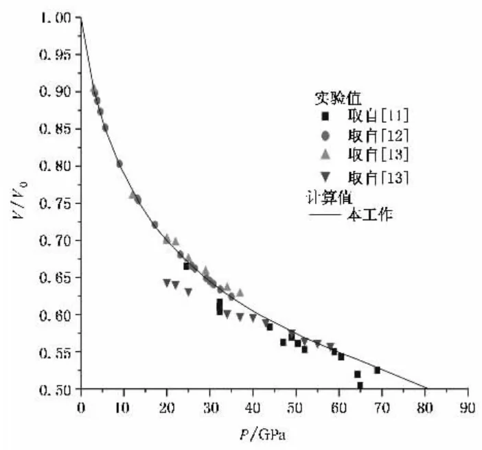
Relative Density

The original paper mainly contains volume-change curves. Comparing the data at 40 GPa and 0 GPa gives a ratio of about $0.620.62$, while the value from this simulation is $0.7090.709$, which is somewhat high.

Analysis

The simulation results in this tutorial all have a certain degree of error, because this tutorial is only a rough simulation rather than a research article. The main source of error should be the force field: the force field used here was mainly fitted for room-temperature and ambient-pressure conditions, so it has relatively large errors under high-temperature and high-pressure conditions.